Time Domain Reflectometry (TDR)

TDR is a method of fault detection and localisation in electric cables. TDR involves sending a fast-rising pulse down a cable and sampling it at the input. The sampled signal is then analysed to look for reflected signals. From the sampled signal, we can detect the presence of a fault and determine the type of the fault and its point of occurrence. TDR is based on the principle that impedance discontinuities in cables result in reflection of an incident signal. To understand more about reflection of electric signals, I suggest you look at this post: Reflection of Electric Signals in Conductors . Faults introduce impedance discontinuities in cables and, therefore, using TDR, we can detect faults in cables. TDR also finds use in geological studies such as testing soil moisture.

Structure of a TDR system

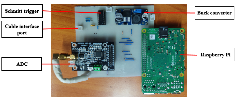
The main parts of a TDR system are a fast-rising pulse generator, a fast-sampling Analogue to Digital Converter (ADC), a processing unit and the Cable Under Test (CUT). Figure 1 shows the architecture of a TDR system.

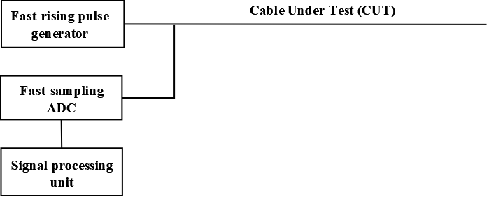
Figure 1: Block diagram of a TDR system.

i. Fast-rising pulse generator

It is used to generate a fast-rising excitation signal. Most TDR systems use rectangular signals as the excitation signal. The signal needs to be fast rising in order to increase the precision of the TDR system.

iI. Fast-sampling Analogue to Digital Converter (ADC)

The ADC is used to digitise the signal at the input port of the CUT. Electric signals travel at the speed close to that of light ($3\times {10}^8$ $m·s^{-1}$). This means that an ADC with a very high sampling rate is required. The output of the ADC is fed to a processing unit for processing.

iii. Processing unit

The processing unit is used to process the sampled signal to detect faults and compute the distance to the faults.

iv. Cable Under Test (CUT)

This is the electric cable being analysed to check for faults.

Principle of operation

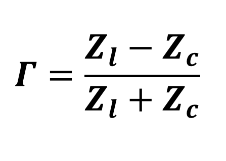
An electric signal travelling down an electric cable gets reflected wholly or partially when it encounters impedance discontinuities in the cable. The reflected signal, $V_r$, is given by:

Where: $\Gamma$ is the reflection coefficient, $Z_c$ is the characteristic impedance of the cable and $Z_l$ is the impedance of the load (fault)

The reflection coefficient is dependent on the impedance of the fault. Faults with impedances higher than the characteristic impedance of the cable have a positive reflection coefficient and, hence, result in reflected signals that are in phase with the incident signal. Conversely, faults with impedances lower than the characteristic impedance of the cable have a negative reflection coefficient and they cause reflected signals that are out of phase with the incident signal. The magnitude of the reflection coefficient is directly proportional to the amplitude of the impedance of the fault. Open circuit and short circuit have the optimum reflection coefficients of $1$ and $-1$ respectively. Therefore, from the magnitude and the phase of the reflected signal, we can tell the type of impedance in a cable.

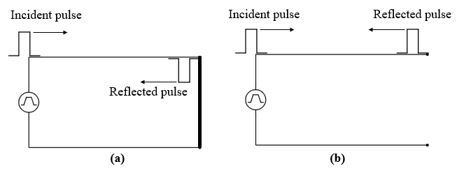
Figure 2: Reflection due to: (a) A short circuit and (b) an open circuit.

To determine the point of occurrence of the fault, the time delay, $△t$, of the reflected signal is used. Electricity travels in an electric cable at the speed close to the speed of light in vacuum. The ratio of the speed of electricity in a conductor to that of light in a vacuum is called the velocity factor, $VF$.

Where $v$ is the velocity of electricity in a cable and $c$ is the speed of light in vacuum.

Different cables have different velocity factors. The speed of an electric signal is computed from the velocity factor. Using the known speed of the signal, and the time delay of the reflected signal, the distance to the point of the fault, $d_f$, is given by:

Therefore, by sending a fast-rising pulse down a cable, sampling it at the input port and analysing it, we can detect faults in cables, determine the type of fault and also compute the distance from the input to the point of the fault.